MNIST From Scratch Using NumPy

To gain a deeper understanding of what is happening in Neural Networks I decided I wanted to complete a project froms scratch without the help of Pytorch or Tensorflow. The best part about machine learning is the easiest way to learn is by training models! Therefore I am going to train as many as I possibly can throughout this journey to master Artifical Intelligence!

This is the training process I will be going through:

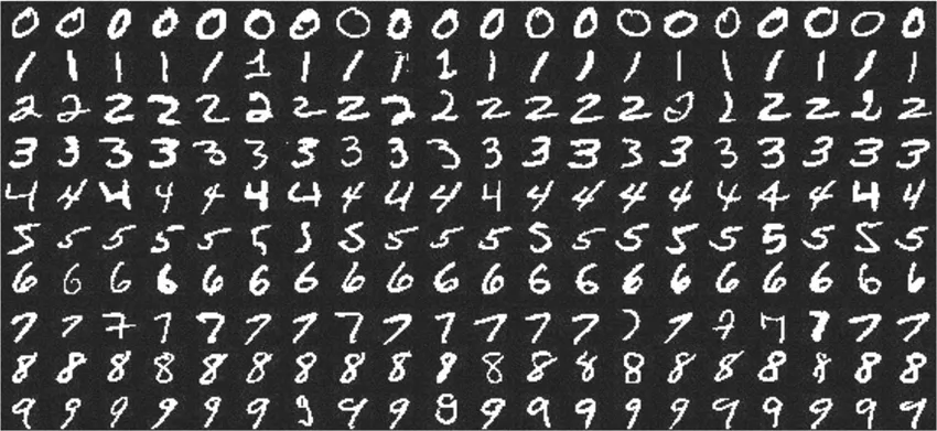
This is the dataset I will be using:

Code Implementation

Prep Data

import numpy as np
import matplotlib.pyplot as plt

def load_data(path):
    def one_hot(y):
        table = np.zeros((y.shape[0], 10))
        for i in range(y.shape[0]):
            table[i][int(y[i][0])] = 1 
        return table

    def normalize(x): 
        x = x / 255
        return x 

    data = np.loadtxt('{}'.format(path), delimiter = ',', skiprows=1)
    return normalize(data[:,1:]),one_hot(data[:,:1])


X_train, y_train = load_data('mnist_train.csv')
X_test, y_test = load_data('mnist_test.csv')

Setup Neural Network

import seaborn as sns
from sklearn.metrics import confusion_matrix

class NeuralNetwork:
    def __init__(self, X, y, hidden_sizes=(256, 128), batch=64, lr=.008, epochs=75):
        self.X_train, self.y_train = X, y  # training data

        # Parameters
        self.batch = batch
        self.lr = lr
        self.epochs = epochs

        # Initialize weights and biases
        input_dim = X.shape[1]
        output_dim = y.shape[1]
        self.sizes = [input_dim, *hidden_sizes, output_dim]

        self.weights = []
        self.biases = []
        for i in range(len(self.sizes) - 1):
            # Xavier/Glorot Initialization for weights
            bound = np.sqrt(6. / (self.sizes[i] + self.sizes[i+1]))
            self.weights.append(np.random.uniform(-bound, bound, (self.sizes[i], self.sizes[i+1])))
            self.biases.append(np.zeros((1, self.sizes[i+1])))

        # List to store loss and accuracy history
        self.train_loss, self.train_acc = [], []

    def ReLU(self, x):
        return np.maximum(0, x)

    def dReLU(self, x):
        return (x > 0).astype(float)

    def softmax(self, x):
        e_x = np.exp(x - np.max(x, axis=1, keepdims=True))
        return e_x / np.sum(e_x, axis=1, keepdims=True)

    def cross_entropy(self, pred, real):
        n_samples = real.shape[0]
        res = pred - real
        return res/n_samples

    def error(self, y_pred, y_real):
        return -np.sum(y_real * np.log(y_pred))

    def feedforward(self, X):
        self.a = [X]
        self.z = []
        for i in range(len(self.sizes) - 2):
            self.z.append(np.dot(self.a[-1], self.weights[i]) + self.biases[i])
            self.a.append(self.ReLU(self.z[-1]))
        self.z.append(np.dot(self.a[-1], self.weights[-1]) + self.biases[-1])
        self.a.append(self.softmax(self.z[-1]))
        return self.a[-1]
    
    def backprop(self, y):
        m = y.shape[0]
        dw = []  # dC/dW
        db = []  # dC/dB
        dz = [self.cross_entropy(self.a[-1], y)]  # dC/dz 

        # loop through each layer in reverse order
        for i in reversed(range(len(self.sizes) - 1)):
            dw.append(np.dot(self.a[i].T, dz[-1]) / m)
            db.append(np.sum(dz[-1], axis=0, keepdims=True) / m)
            if i > 0:  # Skip dz for input layer
                da = np.dot(dz[-1], self.weights[i].T)
                dz.append(da * self.dReLU(self.z[i-1]))

        # Reverse lists since we computed in reverse
        self.dw = dw[::-1]
        self.db = db[::-1]

    def update_weights(self):
        for i in range(len(self.sizes) - 1):
            self.weights[i] -= self.lr * self.dw[i]
            self.biases[i] -= self.lr * self.db[i]

    def train(self):
        for epoch in range(self.epochs):
            # Forward and Backward pass for each batch
            for i in range(0, self.X_train.shape[0], self.batch):
                X = self.X_train[i:i+self.batch]
                y = self.y_train[i:i+self.batch]
                self.feedforward(X)
                self.backprop(y)
                self.update_weights()

            # Save and print loss and accuracy at the end of each epoch
            train_pred = self.feedforward(self.X_train)
            train_loss = self.error(train_pred, self.y_train)
            self.train_loss.append(train_loss)
            train_acc = np.mean(np.argmax(self.y_train, axis=1) == np.argmax(train_pred, axis=1))
            self.train_acc.append(train_acc)
            print(f"Epoch {epoch+1}/{self.epochs} - loss: {train_loss:.4f} - acc: {train_acc:.4f}")


    def plot_loss(self):
        plt.figure(figsize=(10, 6))
        plt.plot(self.train_loss, label='Train Loss')
        plt.title("Loss vs. Epochs")
        plt.xlabel("Epochs")
        plt.ylabel("Loss")
        plt.legend()
        plt.grid(True)
        plt.show()

    def plot_acc(self):
        plt.figure(figsize=(10, 6))
        plt.plot(self.train_acc, label='Train Accuracy')
        plt.title("Accuracy vs. Epochs")
        plt.xlabel("Epochs")
        plt.ylabel("Accuracy")
        plt.legend()
        plt.grid(True)
        plt.show()

    def plot_confusion_matrix(self, X_test, y_test):
        y_pred = self.feedforward(X_test)
        y_pred = np.argmax(y_pred, axis=1)
        y_true = np.argmax(y_test, axis=1)

        plt.figure(figsize=(10, 6))
        cm = confusion_matrix(y_true, y_pred)
        sns.heatmap(cm, annot=True, fmt='d', cmap='Blues')
        plt.title("Confusion Matrix")
        plt.xlabel("Predicted Label")
        plt.ylabel("True Label")
        plt.show()

    def test(self, X_test, y_test):
        y_pred = self.feedforward(X_test)
        acc = np.mean(np.argmax(y_test, axis=1) == np.argmax(y_pred, axis=1))
        print("Test Accuracy: {:.2f}%".format(100 * acc))

# Assume you have training data X_train, y_train and test data X_test, y_test.
NN = NeuralNetwork(X_train, y_train)
NN.train()
NN.plot_loss()
NN.plot_acc()
NN.test(X_test, y_test)

Epoch 1/75 - loss: 137129.5682 - acc: 0.1268
Epoch 2/75 - loss: 131418.5482 - acc: 0.2510
Epoch 3/75 - loss: 126235.7899 - acc: 0.3750
Epoch 4/75 - loss: 121282.3307 - acc: 0.4682
Epoch 5/75 - loss: 116405.4435 - acc: 0.5308
Epoch 6/75 - loss: 111541.0515 - acc: 0.5762
Epoch 7/75 - loss: 106677.8296 - acc: 0.6109
Epoch 8/75 - loss: 101828.8328 - acc: 0.6406
Epoch 9/75 - loss: 97028.6175 - acc: 0.6657
Epoch 10/75 - loss: 92318.4315 - acc: 0.6870
Epoch 11/75 - loss: 87754.4193 - acc: 0.7048
Epoch 12/75 - loss: 83385.3926 - acc: 0.7205
Epoch 13/75 - loss: 79251.8938 - acc: 0.7342
Epoch 14/75 - loss: 75378.7727 - acc: 0.7472
Epoch 15/75 - loss: 71773.3357 - acc: 0.7584
Epoch 16/75 - loss: 68437.6353 - acc: 0.7689
Epoch 17/75 - loss: 65362.9476 - acc: 0.7790
Epoch 18/75 - loss: 62536.8781 - acc: 0.7874
Epoch 19/75 - loss: 59943.4454 - acc: 0.7947
Epoch 20/75 - loss: 57565.2254 - acc: 0.8012
Epoch 21/75 - loss: 55384.5291 - acc: 0.8075
Epoch 22/75 - loss: 53382.6301 - acc: 0.8124
Epoch 23/75 - loss: 51543.0992 - acc: 0.8176
Epoch 24/75 - loss: 49850.6227 - acc: 0.8219
Epoch 25/75 - loss: 48290.0803 - acc: 0.8257
Epoch 26/75 - loss: 46848.8197 - acc: 0.8291
Epoch 27/75 - loss: 45515.0078 - acc: 0.8325
Epoch 28/75 - loss: 44278.3199 - acc: 0.8354
Epoch 29/75 - loss: 43129.9729 - acc: 0.8380
Epoch 30/75 - loss: 42061.1922 - acc: 0.8404
Epoch 31/75 - loss: 41065.1078 - acc: 0.8430
Epoch 32/75 - loss: 40135.0729 - acc: 0.8456
Epoch 33/75 - loss: 39265.3970 - acc: 0.8477
Epoch 34/75 - loss: 38450.5495 - acc: 0.8498
Epoch 35/75 - loss: 37685.9770 - acc: 0.8516
Epoch 36/75 - loss: 36967.8159 - acc: 0.8534
Epoch 37/75 - loss: 36291.8714 - acc: 0.8550
Epoch 38/75 - loss: 35654.2947 - acc: 0.8566
Epoch 39/75 - loss: 35052.2173 - acc: 0.8580
Epoch 40/75 - loss: 34482.9341 - acc: 0.8598
Epoch 41/75 - loss: 33943.8488 - acc: 0.8615
Epoch 42/75 - loss: 33432.6360 - acc: 0.8630
Epoch 43/75 - loss: 32947.0680 - acc: 0.8644
Epoch 44/75 - loss: 32485.4873 - acc: 0.8657
Epoch 45/75 - loss: 32046.1996 - acc: 0.8672
Epoch 46/75 - loss: 31627.5566 - acc: 0.8687
Epoch 47/75 - loss: 31228.1234 - acc: 0.8698
Epoch 48/75 - loss: 30846.5072 - acc: 0.8710
Epoch 49/75 - loss: 30481.5252 - acc: 0.8721
Epoch 50/75 - loss: 30132.1861 - acc: 0.8730
Epoch 51/75 - loss: 29797.4417 - acc: 0.8741
Epoch 52/75 - loss: 29476.4986 - acc: 0.8750
Epoch 53/75 - loss: 29168.3811 - acc: 0.8758
Epoch 54/75 - loss: 28872.4349 - acc: 0.8767
Epoch 55/75 - loss: 28587.9371 - acc: 0.8776
Epoch 56/75 - loss: 28314.2709 - acc: 0.8784
Epoch 57/75 - loss: 28050.7225 - acc: 0.8793
Epoch 58/75 - loss: 27796.8310 - acc: 0.8801
Epoch 59/75 - loss: 27552.0479 - acc: 0.8808
Epoch 60/75 - loss: 27315.8496 - acc: 0.8816
Epoch 61/75 - loss: 27087.7822 - acc: 0.8822
Epoch 62/75 - loss: 26867.4438 - acc: 0.8829
Epoch 63/75 - loss: 26654.5043 - acc: 0.8834
Epoch 64/75 - loss: 26448.5684 - acc: 0.8840
Epoch 65/75 - loss: 26249.2325 - acc: 0.8849
Epoch 66/75 - loss: 26056.2143 - acc: 0.8855
Epoch 67/75 - loss: 25869.1442 - acc: 0.8863
Epoch 68/75 - loss: 25687.7101 - acc: 0.8869
Epoch 69/75 - loss: 25511.7632 - acc: 0.8876
Epoch 70/75 - loss: 25340.9962 - acc: 0.8881
Epoch 71/75 - loss: 25175.1319 - acc: 0.8885
Epoch 72/75 - loss: 25014.0458 - acc: 0.8890
Epoch 73/75 - loss: 24857.4101 - acc: 0.8895
Epoch 74/75 - loss: 24704.9976 - acc: 0.8898
Epoch 75/75 - loss: 24556.6116 - acc: 0.8904

Test Accuracy: 89.78%

NN.plot_confusion_matrix(X_test, y_test)

Conclusion

This was a fun project where I created a 3-layer Neural-Net only using Numpy! The model performed very well. It finished with 89.78% accuracy! I found it very intresting that the model’s most common mistake was confusing 5’s for 3’s! The confusion matrix does confirm that model was very consistent on all numbers!

Being able to see the model at such a low level allowed me to look at Neural Nets from a mathmatical standpoint which helped me understand the “Black-Box” in an insightful way! Matrix Multiplcations truly are incredible!